Predict California House Prices

Introduction

In Machine Learning, Regression is a set of statistical processes for estimating the relationships between dependant variables. Its primary goal is to forecast or predict a value of y given a set of other variables. In contrast to Classification where the outcome is a discrete number or class, Regression yields a continuous number. Say for example tomorrow’s weather forecast 33.4°C.

In this post, we’ll tackle one of the most famous Regression problems in Machine Learning. Namely, The California House Price Prediction problem. It is the “Hello, World!” of Regression Analysis, and by the end you should have a comprehensive understanding of the common steps needed to solve Regression problems.

Frame the Problem

We are going to use California census data to build a model of housing prices in the state. This data includes metrics; such as, the population, median income, and median housing price for each block group in California.

Block groups are the smallest geographical unit for which the US Census Bureau publishes sample data (a block group typically has a population of 600 to 3,000 people). We will call them “districts” for short.

Your model should learn from this data and be able to predict the median housing price in any district, given all the other metrics. Since our model is going to learn from labeled historical data, then this falls under the Supervised Learning category of the Machine Learning domain.

Understanding the Data

We’ll use the California Housing Prices dataset from the StatLib repository¹. This dataset is based on data from the 1990 California census. It is not exactly recent! But it has many qualities for learning, so we will pretend it is recent data for the sake of learning.

Let’s load the data using Pandas and take a look at the top five rows using the DataFrame’s head() method.

# coding: utf-8
import os
import pandas as pd

# Data path
HOUSING_PATH = os.path.join("data", "housing.csv")

# Load housing data into a pandas dataframe and view the top 5 rows
housing_df = pd.read_csv(HOUSING_PATH)
housing_df.head()

Each row represents one district. There are 10 attributes:

1. Longitude
2. Latitude
3. House Median Age
4. Total Rooms
5. Total Bedrooms
6. Population
7. Households
8. Median Income
9. Median House Value
10. Ocean Proximity

The info() method is useful to get a quick description of the data, in particular the total number of rows, each attribute’s type, and the number of non-null values.

# Show quick description of the data
housing_df.info()

There are 20,640 entries in the dataset, which means that it is fairly small by Machine Learning standards, but it’s perfect to get started. Notice that the total_bedrooms attribute has only 20,433 non-null values, meaning that 207 districts are missing this feature. We will need to take care of this later.

All attributes are numerical, except the ocean_proximity field. Its type is object, so it could hold any kind of Python object. But since you loaded this data from a CSV file, you know that it must be a text attribute. When you looked at the top five rows, you probably noticed that the values in the ocean_proximity column were repetitive, which means that it is probably a categorical attribute. You can find out what categories exist and how many districts belong to each category by using the value_count() method.

# Show unique values of the categorical field
housing_df["ocean_proximity"].value_counts()

Let’s look at other fields. The describe() method shows a summary of the numerical attributes.

# Show summary of all numercial values
housing_df.describe()

The count, mean, min, and max rows are self-explanatory. Note that the null values are ignored (so, for example, the count of total_bedrooms is 20,433, not 20,460). The std shows the standard deviation, which measures how dispersed the values are². The 25%, 50%, and 75% rows show the corresponding percentiles. A percentile indicates the value below which a given percentage of observations in a group of observations fall. For example, 25% of the districts have a housing_median_age lower than 18, while 50% are lower than 29 and 75% are lower than 37. These are often called the 25th percentile (or first quartile), the median, and the 75th percentile (or third quartile).

A quick way to get a feel of the type of data you are dealing with is to plot a histogram for each numerical attribute. A histogram shows the number of instances (on the vertical axis) that have a given value range (on the horizontal axis). You can either plot this one attribute at a time, or you can call the hist()³ method on the whole dataset, and it will plot a histogram for each numerical attribute.

housing_df.hist(bins=50, figsize=(20, 15))
plt.show()

There are a few things you might notice in these histograms:

1. First, the median income attribute does not look like it is expressed in US dollars (USD). This is because the data has been scaled and capped at 15 (actually, 15.0001) for higher median incomes, and at 0.5 (actually, 0.4999) for lower median incomes. The numbers represent roughly tens of thousands of dollars (e.g., 3 actually means about $30,000). Working with preprocessed attributes is common in Machine Learning and it is not necessarily a problem, but you should always try to understand how the data was computed.
2. The housing median age and the median house value were also capped. The latter may be a serious problem since it is your target attribute (your labels). Your Machine Learning algorithms may learn that prices never go beyond that limit.
3. These attributes have very different scales. We will discuss this later.
4. Finally, many histograms are tail-heavy: they extend much farther to the right of the median than to the left. This may make it a bit harder form some Machine Learning algorithms to detect patterns. We will try transforming these attributes later on to have a more bell-shaped distribution.

Hopefully you now have a better understanding of the kind of data you’re dealing with.

Create a Test Set

It may sound weird to voluntarily set aside part of the data at this stage. After all, you have only taken a quick glance at the data, and surely you should learn a whole lot more about it before you decide what algorithms to use, right?

This is true, but your brain is an amazing pattern detection system, which means that it is highly prone to overfitting: if you look at the test set, you may stumble upon some seemingly interesting pattern that leads you to select a particular kind of Machine Learning model. This is called data snooping bias.

Random Sampling

Creating a test set is theoretically simple. Pick some instances randomly, typically 20% of the dataset (or less if your dataset is very large), and set them aside.

import numpy as np

def split_train_test(data, test_ratio):
        shuffled_indices = np.random.permutation(len(data))
        test_set_size = int(len(data) * test_ratio)
        test_indices = shuffled_indices[:test_set_size]
        train_indices = shuffled_indices[test_set_size:]
        return data.iloc[train_indices], data.iloc[test_indices]

You can then use this function like this.

>>> train_set, test_set = split_train_test(housing_df, 0.2)
>>> len(train_set)
16512
>>> len(test_set)
4128

Well, this works, but it is not perfect. If you run this function again, it will generate a different test set! Over time, you (or your Machine Learning algorithms) will get to see the whole dataset, which is what you want to avoid.

One solution is to save the test set on the first run and then load it in subsequent runs. Another option is to set the random number generator’s seed (e.g., with np.random.seed(42))⁴ before calling np.random.permutation() so that it always generates the same shuffled indices.

Scikit-Learn provides a few functions to split datasets into multiple subsets in various ways. The simplest function is train_test_split() which does pretty much the same thing as our function split_train_test() with a couple of additional features.

First, there is a random_state parameter that allows you to set the random generator seed. Second, you can pass it multiple datasets with an identical number of rows, and it will split them on the same indices (this is very useful, for example, if you have a separate DataFrame for labels).

from sklearn.model_selection import train_test_split

train_set, test_set = train_test_split(housing_df, test_size=0.2, random_state=42)

So far we have considered purely random sampling methods. This is generally fine if your dataset is large enough (especially relative to the number of attributes), but if it is not , you run the risk of introducing a significant sampling bias.

Stratified Sampling

When a survey company decides to call 1,000 people to ask them a few questions, the don’t just pick 1,000 people randomly from a phone book. They try to ensure that these 1,000 people are representative of the whole population. For example, the US population is 51.3% females and 48.7% males, so a well-conducted survey in the US would try to maintain this ratio in the sample: 513 female and 487 male. This is called stratified sampling , where the population is divided into homogeneous subgroups called strata, and the right number of instances are sampled from each stratum to guarantee that the test set is representative of the overall population.

Suppose you spoke to experts who told you that the median income is a very important attribute to predict median housing prices. You may want to ensure that the test set is representative of the various categories of incomes in the whole dataset. Since the median income is a continuous numerical attribute, you first need to create an income category attribute.

Let’s look at the median income histogram more closely.

housing_df["median_income"].hist()

Most median income values are clustered around 1.5 to 6 (i.e., $15,000-$60,000), but some median incomes go far beyond 6. It is important to have a sufficient number of instances in your dataset for each startum, or else the estimate of a stratum’s importance may be biased. This means you should not have too many strata, and each stratum should be large enough.

The following code uses the pd.cut() function to create an income category attribute with five categories (labeled from 1 to 5). Category 1 ranges from 0 to 1.5 (i.e., less than $15,000), category 2 from 1.5.to 3 and so on.

housing_df["income_cat"] = pd.cut(
        housing_df["median_income"],
        bins=[0., 1.5, 3.0, 4.5, 6., np.inf],
        labels=[1, 2, 3, 4, 5]
)
housing_df["income_cat"].hist()
plt.show()

Now you are ready to do stratified sampling based on the income category. For this you can use Scikit-Learn’s StratifiedShuffleSplit class.

from sklearn.model_selection import StratifiedShuffleSplit

split = StratifiedShuffleSplit(n_splits=1, test_size=0.2, random_state=42)
for train_index, test_index in split.split(housing_df, housing_df["income_cat"]):
        strat_train_set = housing_df.loc[train_index]
        strat_test_set = housing_df.loc[test_index]

Let’s see if this worked as expected. You can start by looking at the income category proportions in the test set.

If we compare the stratified ratios to the complete dataset we find that they are almost identical.

Now you should remove the income_cat attribute so the data is back to its original state.

for set_ in (strat_train_set, strat_test_set):
        set_.drop("income_cat", axis=1, inplace=True)

We’ve spent quite a bit of time on test set generation for a good reason. This is an often neglected but critical part of a Machine Learning project. Moreover, many of these ideas will be useful later when we discuss cross-validation.

Visualize the Data

So far we have only taken a quick glance at the data to get a general understanding of the kind of data we are manipulating. Now the goal is to go into a little more depth.

First, let’s make sure we have put the test set aside and are only exploring the training set. Also, if the training set is very large, we may want to sample an exploration set, to make manipulations easy and fast. In our case, the set is quite small, so we can just work directly on the full training set. Let’s create a copy so that we can play with it without accidentally modifying the training set.

housing_df = strat_train_set.copy()

Since there is geographical information (latitude and longitude), it is a good idea to create a scatter plot of all districts to visualize the data.

housing_df.plot(kind="scatter", x="longitude", y="latitude")
plt.show()

This seems to be right! However, it is hard to see any particular pattern. We can set the alpha option to 0.1 to make it easier to visualize places where there is high density of data points.

housing_df.plot(kind="scatter", x="longitude", y="latitude", alpha=0.1)
plt.show()

Now that’s much better. You can clearly see the high-density areas. Our brains are very good at spotting patterns in pictures, but you may need to play around with visualization parameters⁵ to make the patterns stand out.

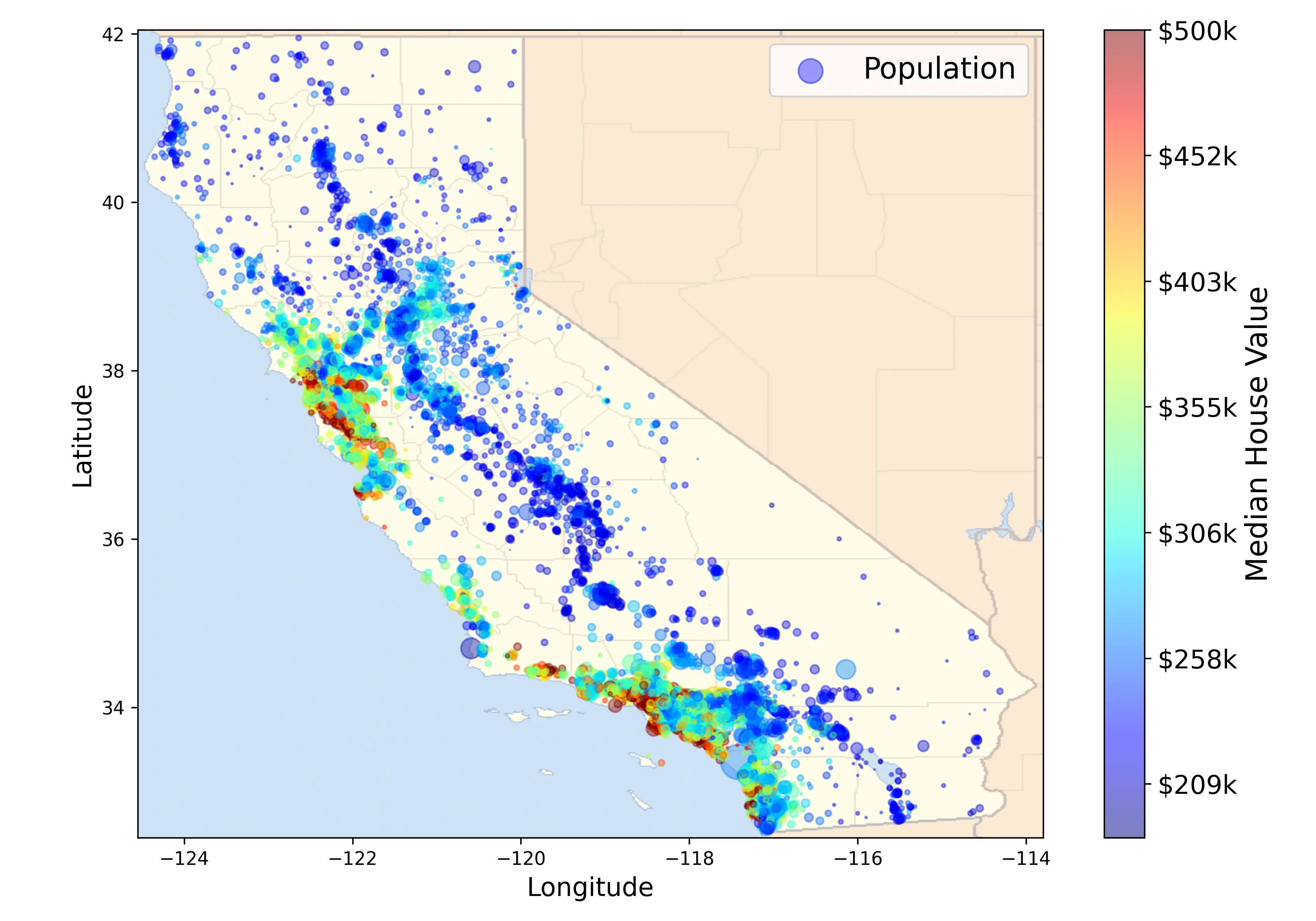
housing_df.plot(
        kind="scatter",
        x="longitude",
        y="latitude",
        alpha=0.4,
        s=housing_df["population"]/100,     # Marker size
        c="median_house_value",             # Marker color
        label="population",
        cmap=plt.get_cmap("jet"),           # Colormap
        colorbar=True,
        figsize=(10, 7),
)
plt.legend()
plt.show()

If we look at the housing prices figure above, we can see that the radius of each circle marker represents the district’s population (option s), and the color of each marker represents the price (option c). We also use a predefined color map (option cmap) called jet, which ranges from blue (low values) to red (high prices).

Let’s redraw our scatter plot once again, but with an image of California as the background⁶.

This looks like California all right! You can clearly see the high-density areas around the Bay Area and around Los Angeles and San Diego, plus a long line of fairly high density in the Central Valley.

Looking for Correlations

Since the dataset is not too large, we can easily compute the standard correlation coefficient (also called Pearson’s r) between every pair of attributes using the corr() method.

corr_matrix = housing_df.corr(numeric_only=True)

Now let’s look at how much each attribute correlates with the median house value.

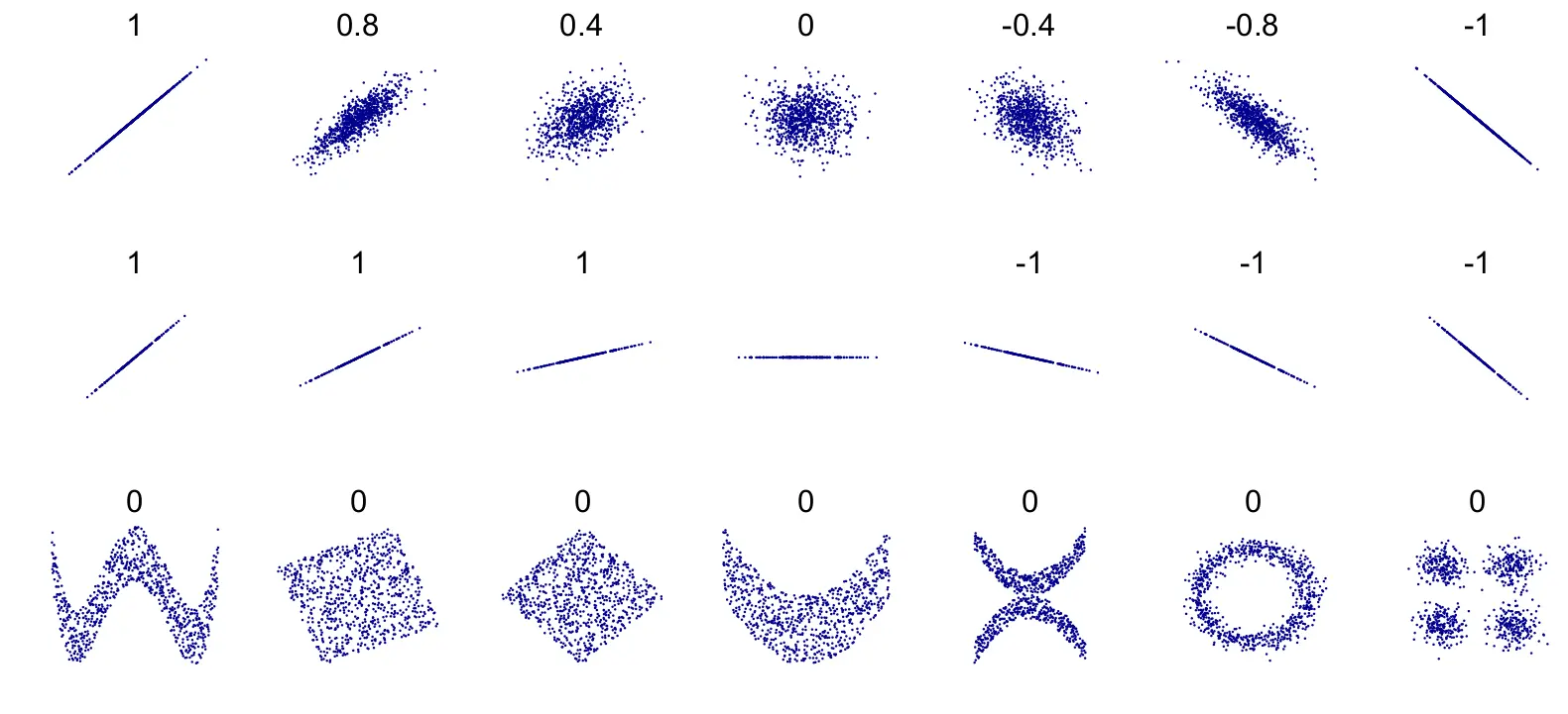
The correlation coefficient ranges from -1 to 1. When it is close to 1, it means that there is a strong positive correlation; for example, the median house value tends to go up when the media income goes up. When the coefficient is close to -1, it means that there is a strong negative correlation. You can see a small negative correlation between the latitude and the median house value (i.e., prices have a slight tendency to go down when you go north). Finally, coefficients close to 0 mean that there is no linear correlation.

Another way to check for correlation between attributes is to use the pandas scatter_matrix() function, which plots every numerical attribute against every other numerical attribute. Since there are now 11 numerical attributes, you would get \(11^{2} = 121\) plots, which would not fit on a page. Let’s just focus on a few promising attributes that seem most correlated with the median housing value.

from pandas.plotting import scatter_matrix

attributes = ["median_house_value", "median_income", "total_rooms", "housing_median_age"]
scatter_matrix(housing_df[attributes], figsize=(12, 8))

The main diagonal (top left to bottom right) would be full of straight lines if pandas plotted each variable against itself, which would not be very useful. So instead pandas displays a histogram of each attribute (other options are available; see the pandas documentation for more details).

The most promising attribute to predict the median house value is the median income, so let’s zoom in on their correlation scatter plot.

housing_df.plot(kind="scatter", x="median_income", y="median_house_value", alpha=0.1)

The plot reveals a few things. First, the correlation is indeed very strong. You can clearly see the upward trend, and the points are not too dispersed. Second, the price cap that we noticed earlier is clearly visible as a horizontal line at $500,000. But this plot reveals other less obvious straight lines: a horizontal line around $450,000, another around $350,000, perhaps one around $280,000, and a few more below that. You may want to try removing the corresponding districts to prevent your algorithms from learning to reproduce these data quirks.

Experimenting with Attribute Combinations

One last thing you might want to do before preparing the data for Machine Learning algorithms is to try out various attribute combinations. For example, the total number of rooms in a district is not very useful if you don’t know how many households there are. What you really want is the number of rooms per household. Similarly, the number of bedrooms by itself is not very useful. You probably want to compare it to the total number of rooms. And the population per household also seems like an interesting attribute combination to look at. Let’s create these attributes.

housing_df["rooms_per_household"] = housing_df["total_rooms"] / housing_df["households"]
housing_df["bedrooms_per_room"] = housing_df["total_bedrooms"] / housing_df["total_rooms"]
housing_df["population_per_household"] = housing_df["population"] / housing_df["households"]

corr_matrix = housing_df.corr(numeric_only=True)
corr_matrix["median_house_value"].sort_values(ascending=False)

The new bedrooms_per_room attribute is much more correlated with the median house value than the total number of rooms or bedrooms. Apparently houses with a lower bedroom/room ratio tend to be more expensive. The number of rooms per household is also more informative than the total number of rooms in a district. Obviously the larger the house, the more expensive it is.

This round of exploration does not have to be absolutely thorough. The point is to start off on the right foot and quickly gain insights that will help you get a first reasonably good prototype. But this is an iterative process. Once you get a prototype up and running, you can analyze its output to gain more insights and come back to this exploration step again.

Prepare the Data for Machine Learning Algorithms

It’s time to prepare the data for our Machine Learning algorithms. Instead of doing this manually, we should write functions for this purpose, for several good reasons:

• This will allow us to reproduce these transformations easily on any dataset (e.g., the next time we get a fresh dataset).
• We will gradually build a library of transformation functions that we can reuse in future projects.
• We can use these functions in our live system to transform the new data before feeding it to our algorithms.
• This will make it possible to easily try out various transformations and see which combination of transformations work best.

But first let’s revert to a clean training set (by copying strat_train_set once again). Let’s also separate the predictors and the labels, since we don’t necessarily want to apply the same transformations to the predictors and the target values (note that drop() creates a copy of the data and does not affect strat_train_set).

housing_df = strat_train_set.drop("median_house_value", axis=1)
housing_labels = strat_train_set["median_house_value"].copy()

Now we have a fresh and clean training set along with the prediction labels.

Data Cleaning

Most Machine Learning algorithms cannot work with missing features, so let’s create a few functions to take care of them. We saw earlier that the total_bedrooms attribute has some missing values, so let’s fix this. We have three options:

1. Get rid of the corresponding districts.
2. Get rid of the whole attribute.
3. Set the missing values to some value (zero, the mean, the median, etc.).

We can accomplish these easily using DataFrams’s dropna(), drop(), and fillna() methods:

# option 1
housing_df.dropna(subset=["total_bedrooms"])

# option 2
housing_df.drop("total_bedrooms", axis=1)

# option 3
median = housing_df["total_bedrooms"].median()
housing_df["total_bedrooms"] = housing_df["total_bedrooms"].fillna(median)

If we choose option 3, we should compute the median value on the training set and use it to fill the missing values in the training set. Don’t forget to save the median value that you have computed. We will need it later to replace missing values in the test set when you want to evaluate the system.

On the other hand, Scikit-Learn provides a handy class to take care of missing values, namely SimpleImputer. Here is how to use it. First, we need to create a SimpleImputer instance, specifying that we want to replace each attribute’s missing values with the median of that attribute.

from sklearn.impute import SimpleImputer

imputer = SimpleImputer(strategy="median")

Since the median can only be computed on numerical attributes, we need to create a copy of the data without the text attribute ocean_proximity.

housing_num = housing_df.drop("ocean_proximity", axis=1)

Now you can fit the imputer instance to the training data using the fit() method.

imputer.fit(housing_num)

The imputer has simply computed the median of each attribute and stored the result in its statistics_ instance variable. Only the total_bedrooms attribute had missing values, but we cannot be sure that there won’t be any missing values in new data after the system goes live, so it is safer to apply the imputer to all the numerical attributes.

Now we can use this “trained” imputer to transform the training set by replacing missing values with the learned medians.

X = imputer.transform(housing_num)

The result is a plain NumPy array containing the transformed features. If you want to put it back into a pandas DataFrame, it’s simple.

housing_df = pd.DataFrame(X, columns=housing_num.columns, index=housing_num.index)

Now we have filled in all missing values for the total_bedrooms attribute with the median value of that attribute column.

Handling Text and Categorical Attributes

So far we have only dealt with numerical attributes, but now let’s look at text attributes. In this dataset, there is just one, the ocean_proximity attribute. Let’s look at its value for the first 10 instances.

housing_cat = strat_train_set[["ocean_proximity"]]
housing_cat.head(10)

The ocean_proximity attribute is not arbitrary text. There limited number of possible values, each of which represents a category. So this attribute is a categorical attribute. Most Machine Learning algorithms prefer to work with numbers, so let’s convert these categories from text to numbers. For this, we can use Scikit-Learn’s OrdinalEncoder class⁷.

from sklearn.preprocessing import OrdinalEncoder

ordinal_encoder = OrdinalEncoder()
housing_cat_encoded = ordinal_encoder.fit_transform(housing_cat)
housing_cat_encoded[:10]

You can get the list of categories using the categories_ instance variable. It is a list containing a 1D array of categories for each categorical attribute (in this case, a list containing a single array since there is just one categorical attribute).

ordinal_encoder.categories_

One issue with this representation is that ML algorithms will assume that two nearby values are more similar than two distant values. This may be fine in some cases (e.g., for ordered categories such as “bad”, “average”, “good” and “excellent”), but it is obviously not the case for the ocean_proximity column (for example, categories 0 and 4 are clearly more similar than categories 0 and 1).

To fix this issue, a common solution is to create one binary attribute per category. One attribute equal to 1 when the category is <1H OCEAN (and 0 otherwise), another attribute equal to 1 when the category is INLAND (and 0 otherwise), and so on. This is called one-hot encoding because only one attribute will be equal to 1 (hot), while the others will be 0 (cold). The new attributes are sometimes called dummy attributes. Scikit-Learn provides a OneHotEncoder class to convert categorical values into one-hot vectors⁸.

from sklearn.preprocessing import OneHotEncoder

cat_encoder = OneHotEncoder()
housing_cat_1hot = cat_encoder.fit_transform(housing_cat)
housing_cat_1hot

Notice that the output is a SciPy sparse matrix, instead of a NumPy array. This is very useful when you have categorical attributes with thousands of categories. After one-hot encoding, we get a matrix with thousands of columns, and the matrix is full of 0s except for a single 1 per row. Using up tons of memory mostly to store zeros would be very wasteful, so instead a sparse matrix only stores the location of the nonzero elements. You can use it mostly like a normal 2D array⁹, but if you really want to convert it to a (dense) NumPy array, just call the toarray() method.

Once again, you can get the list of categories using the encoder’s categories_ instance variable.

cat_encoder.categories_

Footnotes